l   Development of Camera Calibration Field

The purpose of camera calibration is to mathematically describe the internal geometry of the imaging system, particularly after a light ray passes through the camera’s perspective center. In order to determine such internal characteristics, a self-calibrating bundle adjustment method with additional parameters is adopted [28,29] that can automatically recognize and measure the image coordinates of retro-reflective coded targets. Based on this functionality, we develop a rotatable round table surmounted by 112 pillars. The coded targets are then fixed to the top of the pillars and the table surface to establish a three-dimensional calibration field with heights varying from 0 to 30 cm. Instead of changing the camera location during image acquisition, the table is simply rotated. Moreover, the camera’s viewing direction is inclined 30°~45° with respect to the table’s surface normal. The concept for the acquisition of convergent geometry by means of a rotatable calibration field is illustrated in Figure 1. The round table is rotated at 45° intervals while capturing the calibration images. This results in 8 images with convergent angles of 60° to 90°, which is a strong convergent imaging geometry. In order to decouple the correlation between IOPs and EOPs during least-squares adjustment, it is suggested that an additional eight images be acquired with the camera rotated for portrait orientation, i.e., change roll angle with 90°. Finally, for the purpose of increasing image measurement redundancy, two additional images (landscape and portrait) are taken with the camera’s optical axis perpendicular to the table surface.

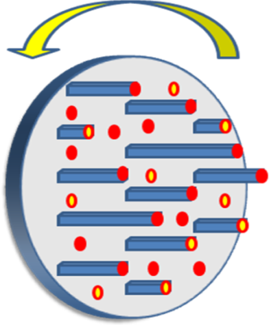
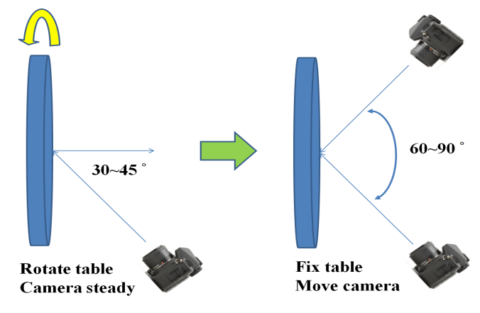
Figure 1. Single camera calibration using a rotatable calibration field.

The relative position of all the code targets is firmly fixed and remains stationary during rotation. This is essentially the same as surrounding the calibration field and taking pictures, introducing a ring type convergent imaging geometry. The proposed ring type configuration is difficult to obtain with a fixed calibration field and particularly for a limited space where the floor and ceiling will constrain the camera’s location. A sample image for camera calibration is illustrated in Figure 2. One may observe that the coded targets are well spread out to the whole image frame, especially the image corners, where the most critical regions to describe the radial lens distortion are. In the figure, the bigger white dots are designed for low resolution cameras to increase the number of tie-point measurements by the auto-referencing function. The auto-referencing is performed by predicting the detected white dots from one image to the others using epipolar geometry in case the relative orientation has been established in advance by means of code targets. Meanwhile, Figure 3 also shows two enlarged code targets. In each coded target, two distance observables are constructed by four white points and utilized for scaling purposes during bundle adjustment. This means that the absolute positioning accuracy can be estimated for the calibrated IOPs. Figure 3 depicts the result of bundle convergence for one target from all cameras. The results demonstrate that it is possible to obtain a strong imaging geometry by means of the proposed arrangement.

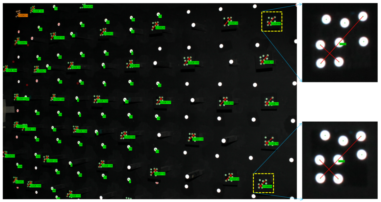
Figure 2. A sample image for camera calibration and two enlarged code targets.

 

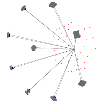
Figure 3. Convergent bundles during camera calibration.

l   Determination of Additional Parameters (APs)

Two approaches for determining the most significant APs are suggested in this study. The first one is to check the change of square root of the a posteriori variance (σ₀) value, which is a measure of the quality of fit between the observed image coordinates and the predicted image coordinates using the estimated parameters (i.e., image residuals), by adding one additional parameter at a time. The predicted image coordinates consider the collinearity among object point, perspective center, and image point by correcting the lens distortion. Thus, if a significant reduction in σ₀ was obtained, for example 0.03 pixels, which is the expected accuracy of image coordinate measurement by the automatic centroid determination method [30], the added parameter is considered as significant one because it correct the image coordinates displacement effectively. Otherwise, it can be ignored. This procedure is simpler and easier to understand its geometric meaning when compare with the next approach.

The second approach is based on checking the correlation coefficients among the parameters and the ratio between the estimated value and its standard deviation (σ), namely the significance index (t). If two APs have a high correlation coefficient, e.g., more than 0.9, then the one with a smaller significance index can be ignored. However, if the smaller one is larger than a pre-specified threshold, the added parameter can still be considered significant. The threshold for the significance index is determined experimentally, e.g., based on the results from the first approach.

The significance index (t) is formulated in equation (1), which is similar to the formula used for stability analysis, as shown in Equation (2), namely change significance (c), used for verifying the stability of a camera’s internal geometry. Both formulations are based the Student’s test. The significance index (t) is described as:

t = |δi|/qi

(1)

where δ_i is the estimated value for parameter i and q_i is the standard deviation for parameter i [31], thus t has no unit. The variable t is an index for the null-hypothesis that “the i^th AP is not significant” compared to the alternative hypothesis “the i^th AP is significant”. On the other hand, the change significance (c) can be described as:

c = |∇i|/pi

(2)

where ; ∇_i is the change of parameter i between calibration time j and j + 1 and q_i,j is the a-posterior variance of parameter i at camera calibration time j [32], thus c has no unit as well. The variable c is an index for the null-hypothesis that “the i^th AP does not change significantly” compared to the alternative hypothesis that “the i^th AP changed significantly”.

 

A SONY A-850 DSLR camera with SONY SAL50F14 (50 mm) lenses is adopted in this study. The significance test results are summarized in Table 1 and can be examined to illustrate the procedure for determining the most significant APs. In the beginning, all APs are un-fixed during self-calibration bundle adjustment to obtain the correlation coefficients between each other. Compatible with common knowledge, the highest correlation coefficients occurred among K1, K2 and K3, i.e., greater than 0.9. In the first run, we note that the significant indices for K2 and K3 are very low. Since they are highly correlated with K1, they are both ignored. In the second run, K2 and K3 are fixed at zero and the significant indices for P1 and P2 are even lower than for the first run. Thus, they are ignored and fixed at zero at the third run. At the third run, B1 and B2 still have significant indices of 29.7 and 15.8, respectively, which is difficult to determine their significant level. Another approach is thus utilized to determine the significant APs by adding one or two parameters and checking the change of σ₀ after bundle adjustment. In the lower part of Table 1, one may observe that a significant improvement in the accuracy occurs only when K1 is considered. Even adding K2, K3, P1, P2, B1 and B2 step by step, the σ₀ has reduced only 0.01 pixels, which is less than the precision of tie-point image coordinate measurement, and the overall accuracy is only improved by 0.0014 mm. This means that they can all be ignored by keeping only the principal distance (c), the principal point coordinates (xp, yp), and the first radial lens distortion coefficient (K1).

 Table 1. Significance testing for the determination of additional parameters.

run	items	c	xp	yp	K1	K2	K3	P1	P2	B1	B2
1	σ	0.0019	0.0025	0.0015	2.50E-07	1.30E-09	2.00E-12	2.30E-07	1.60E-07	6.40E-06	6.90E-06
	Estimated Value	52.26282	0.120988	-0.05591	5.30E-05	7.37E-09	-1.90E-11	-3.79E-06	-2.64E-06	-1.98E-04	-1.03E-04
	Significant Index	27506.7	48.4	37.3	212.1	5.7	9.5	16.5	16.5	31.0	15.0
2	σ	0.0018	0.0026	0.0015	3.60E-08	4.30E-12	4.30E-15	2.40E-07	1.70E-07	6.60E-06	7.20E-06
	Estimated Value	52.25403	0.12224	-0.05537	5.32E-05	0.00E+00	0.00E+00	-3.69E-06	-2.54E-06	-2.01E-04	-1.02E-04
	Significant Index	29030.0	47.0	36.9	1477.3	0.0	0.0	15.4	14.9	30.4	14.1
3	σ	0.0018	0.0013	0.0013	3.70E-08	4.40E-12	4.40E-15	4.40E-10	4.40E-10	6.80E-06	7.30E-06
	Estimated Value	52.25684	0.087639	-0.06862	5.31E-05	0.00E+00	0.00E+00	0.00E+00	0.00E+00	-2.02E-04	-1.16E-04
	Significant Index	29031.6	67.4	52.8	1436.1	0.0	0.0	0.0	0.0	29.7	15.8

run

c

xp

yp

K1

K2

K3

P1

P2

B1

B2

σ0 (pixels)

Relative Accuracy

Overall Accuracy

1

■

■

■

2.00

1:6,200

0.3275

2

■

■

■

■

0.21

1:67,200

0.0303

3

■

■

■

■

0.21

1:67,800

0.0300

4

■

■

■

■

■

0.21

1:68,000

0.0299

5

■

■

■

■

■

■

0.21

1:68,600

0.0297

6

■

■

■

■

■

■

0.20

1:70,300

0.0289